
GDL-1.0 Foundation of Geometric deep learning
- ashvineek9
- Jun 10, 2021
- 2 min read
Updated: Oct 2, 2023
Euclid laid the foundation of geometry that existed for over 2000 years. With the help of few great scientists N. Lobachevsky, J. Bolyai, C. F. Gauss, and B. Riemann, geometry is described as elliptic or hyperbolic surfaces. With this growing field in geometry, few frequent questions were asked – “What is geometry?” and “What's that define geometry?” In 1872, F. Klein explain geometry in Erlangen. He proposed to study geometry using in-variance i.e., the property that remains the same in some transformation.

Such Euclidean geometry can be formulated as structure (angles, distance, areas). These structures are preserved under rotation and translation. Affine geometry that remains preserved (parallel line) under affine transformation. The final common projective geometry, the intersection is preserved. These structures have come from group theory. For example, the energy is conserved in physic which is explained by a shift-invariance.

CNN:
Applying deep learning (dense) on the geometric images miserably fails. The image pixels (28x28) are stacked into one single vector. If the image is shifted by one pixel, it will generate a completely different single vector. So, it will be exceedingly difficult for a neural network to generalize on these different single vectors of the same image. The Neural Network must learn shift in-variance from data. The number of samples needed to learn increases exponentially. This is one of the geometric phonemes known as the curse of dimensionality. This problem is solved using Convolutional Neural Network (CNN). CNN takes advantage of self-similar structures at different scales. It also takes advantage of Local operations with shared weights, Shift-equivalent convolutional filters, and pooling = shift-invariance. It has O(1) parameters per filter and O(n) complexity per layer.

Spatial graph convolution:
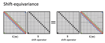
Linear convolution, which is right before non-linear is the linear matching from the input to the output. It is represented as a metric. This is represented as a constant multi-diagonal structure or metrics. This metrics is formed by sifting the version of __ vector using periodic boundary conditions. This metric is called the circulation Metric. In algebra, (metric A) * (metric B) is not = (metric B) * (metric A). In convolution, the two multiplications of circulation metrics will be the same.
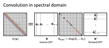
Shift equivarience explains that convolution commutes with the shift. Sift equivalence means the result changes in the same way when the first convolution then shift operation or first shift operation than convolution is applied. Few more points for convolution. Commuting matrices are jointly diagonalizable (same eigenvectors). Eigenvectors of shift operator are the Fourier basis. Fourier bases come from the diagonalization of the shift operations. We can diagonalize convolution by discrete Fourier transform (DFT). Eigenvalues of C(w) are the Fourier transform of w. This finally generates the convolution theorem.
Few key points about convolution. Convolution in the spatial domain is the circulant matrix. Local aggregation with shared parameters. All circulant matrix diagonalized by DFT (eigenvector of shift), apply the element-wise product, apply inverse DFT. Its complexity is O(n) with a small filter and O (n log n) using FFT.


A more detailed explanation for GDL is in the next section of GDL 1.X. Different graphs and convolutions on the graph are explained there. In other sections of GDL 1.X, the applications of GDL are also shown.

Comentários